
Adaptive filter
This article includes a list of general references, but it lacks sufficient corresponding inline citations. (February 2013) |
An adaptive filter is a system with a linear filter that has a transfer function controlled by variable parameters and a means to adjust those parameters according to an optimization algorithm. Because of the complexity of the optimization algorithms, almost all adaptive filters are digital filters. Adaptive filters are required for some applications because some parameters of the desired processing operation (for instance, the locations of reflective surfaces in a reverberant space) are not known in advance or are changing. The closed loop adaptive filter uses feedback in the form of an error signal to refine its transfer function.
Generally speaking, the closed loop adaptive process involves the use of a cost function, which is a criterion for optimum performance of the filter, to feed an algorithm, which determines how to modify filter transfer function to minimize the cost on the next iteration. The most common cost function is the mean square of the error signal.
As the power of digital signal processors has increased, adaptive filters have become much more common and are now routinely used in devices such as mobile phones and other communication devices, camcorders and digital cameras, and medical monitoring equipment.
Example application[edit]
The recording of a heart beat (an ECG), may be corrupted by noise from the AC mains. The exact frequency of the power and its harmonics may vary from moment to moment.
One way to remove the noise is to filter the signal with a notch filter at the mains frequency and its vicinity, but this could excessively degrade the quality of the ECG since the heart beat would also likely have frequency components in the rejected range.
To circumvent this potential loss of information, an adaptive filter could be used. The adaptive filter would take input both from the patient and from the mains and would thus be able to track the actual frequency of the noise as it fluctuates and subtract the noise from the recording. Such an adaptive technique generally allows for a filter with a smaller rejection range, which means, in this case, that the quality of the output signal is more accurate for medical purposes.[1][2]
Block diagram[edit]
The idea behind a closed loop adaptive filter is that a variable filter is adjusted until the error (the difference between the filter output and the desired signal) is minimized. The Least Mean Squares (LMS) filter and the Recursive Least Squares (RLS) filter are types of adaptive filter.
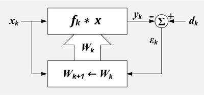
Adaptive Filter. k = sample number, x = reference input, X = set of recent values of x, d = desired input, W = set of filter coefficients, ε = error output, f = filter impulse response, * = convolution, Σ = summation, upper box=linear filter, lower box=adaption algorithm


There are two input signals to the adaptive filter: and which are sometimes called the primary input and the reference input respectively.[3] The adaptation algorithm attempts to filter the reference input into a replica of the desired input by minimizing the residual signal, . When the adaptation is successful, the output of the filter is effectively an estimate of the desired signal.


- which includes the desired signal plus undesired interference and
- which includes the signals that are correlated to some of the undesired interference in .
- k represents the discrete sample number.
The filter is controlled by a set of L+1 coefficients or weights.
- represents the set or vector of weights, which control the filter at sample time k.
- where refers to the 'th weight at k'th time.
- represents the change in the weights that occurs as a result of adjustments computed at sample time k.
- These changes will be applied after sample time k and before they are used at sample time k+1.
![{\displaystyle \mathbf {W} _{k}=\left[w_{0k},\,w_{1k},\,...,\,w_{Lk}\right]^{T}}](https://wikimedia.org/api/rest_v1/media/math/render/svg/927bf9a780012f1a80bb6608a3ff410221a7b43e)


The output is usually but it could be or it could even be the filter coefficients.[4](Widrow)
The input signals are defined as follows:

- where:
- g = the desired signal,
- g' = a signal that is correlated with the desired signal g ,
- u = an undesired signal that is added to g , but not correlated with g or g'
- u' = a signal that is correlated with the undesired signal u, but not correlated with g or g',
- v = an undesired signal (typically random noise) not correlated with g, g', u, u' or v',
- v' = an undesired signal (typically random noise) not correlated with g, g', u, u' or v.

The output signals are defined as follows:
- .
- where:
- = the output of the filter if the input was only g',
- = the output of the filter if the input was only u',
- = the output of the filter if the input was only v'.


Tapped delay line FIR filter[edit]
If the variable filter has a tapped delay line Finite Impulse Response (FIR) structure, then the impulse response is equal to the filter coefficients. The output of the filter is given by
-
- where refers to the 'th weight at k'th time.

Ideal case[edit]
In the ideal case . All the undesired signals in are represented by . consists entirely of a signal correlated with the undesired signal in .


The output of the variable filter in the ideal case is
- .

The error signal or cost function is the difference between and
- . The desired signal gk passes through without being changed.

The error signal is minimized in the mean square sense when is minimized. In other words, is the best mean square estimate of . In the ideal case, and , and all that is left after the subtraction is which is the unchanged desired signal with all undesired signals removed.
![{\displaystyle [u_{k}-{\hat {u}}_{k}]}](https://wikimedia.org/api/rest_v1/media/math/render/svg/cbc75695df122bd9dc20a1832864efec904c1446)


Signal components in the reference input[edit]
In some situations, the reference input includes components of the desired signal. This means g' ≠ 0.
Perfect cancelation of the undesired interference is not possible in the case, but improvement of the signal to interference ratio is possible. The output will be
- . The desired signal will be modified (usually decreased).

The output signal to interference ratio has a simple formula referred to as power inversion.
- .
- where
- = output signal to interference ratio.
- = reference signal to interference ratio.
- = frequency in the z-domain.
- where


This formula means that the output signal to interference ratio at a particular frequency is the reciprocal of the reference signal to interference ratio.[5]
Example: A fast food restaurant has a drive-up window. Before getting to the window, customers place their order by speaking into a microphone. The microphone also picks up noise from the engine and the environment. This microphone provides the primary signal. The signal power from the customer's voice and the noise power from the engine are equal. It is difficult for the employees in the restaurant to understand the customer. To reduce the amount of interference in the primary microphone, a second microphone is located where it is intended to pick up sounds from the engine. It also picks up the customer's voice. This microphone is the source of the reference signal. In this case, the engine noise is 50 times more powerful than the customer's voice. Once the canceler has converged, the primary signal to interference ratio will be improved from 1:1 to 50:1.
Adaptive Linear Combiner[edit]

Adaptive linear combiner showing the combiner and the adaption process. k = sample number, n=input variable index, x = reference inputs, d = desired input, W = set of filter coefficients, ε = error output, Σ = summation, upper box=linear combiner, lower box=adaption algorithm. 
Adaptive linear combiner, compact representation. k = sample number, n=input variable index, x = reference inputs, d = desired input, ε = error output, Σ = summation.


The adaptive linear combiner (ALC) resembles the adaptive tapped delay line FIR filter except that there is no assumed relationship between the X values. If the X values were from the outputs of a tapped delay line, then the combination of tapped delay line and ALC would comprise an adaptive filter. However, the X values could be the values of an array of pixels. Or they could be the outputs of multiple tapped delay lines. The ALC finds use as an adaptive beam former for arrays of hydrophones or antennas.
-
- where refers to the 'th weight at k'th time.

LMS algorithm[edit]
If the variable filter has a tapped delay line FIR structure, then the LMS update algorithm is especially simple. Typically, after each sample, the coefficients of the FIR filter are adjusted as follows:[6]
- for

-
- μ is called the convergence factor.

The LMS algorithm does not require that the X values have any particular relationship; therefore it can be used to adapt a linear combiner as well as an FIR filter. In this case the update formula is written as:

The effect of the LMS algorithm is at each time, k, to make a small change in each weight. The direction of the change is such that it would decrease the error if it had been applied at time k. The magnitude of the change in each weight depends on μ, the associated X value and the error at time k. The weights making the largest contribution to the output, , are changed the most. If the error is zero, then there should be no change in the weights. If the associated value of X is zero, then changing the weight makes no difference, so it is not changed.
Convergence[edit]
μ controls how fast and how well the algorithm converges to the optimum filter coefficients. If μ is too large, the algorithm will not converge. If μ is too small the algorithm converges slowly and may not be able to track changing conditions. If μ is large but not too large to prevent convergence, the algorithm reaches steady state rapidly but continuously overshoots the optimum weight vector. Sometimes, μ is made large at first for rapid convergence and then decreased to minimize overshoot.
Widrow and Stearns state in 1985 that they have no knowledge of a proof that the LMS algorithm will converge in all cases.[7]
However under certain assumptions about stationarity and independence it can be shown that the algorithm will converge if

- where
- = sum of all input power
- where

- is the RMS value of the 'th input

In the case of the tapped delay line filter, each input has the same RMS value because they are simply the same values delayed. In this case the total power is

- where
- is the RMS value of , the input stream.[7]
- where

This leads to a normalized LMS algorithm:
- in which case the convergence criteria becomes: .


Nonlinear Adaptive Filters[edit]
The goal of nonlinear filters is to overcome limitation of linear models. There are some commonly used approaches: Volterra LMS, Kernel adaptive filter, Spline Adaptive Filter [8] and Urysohn Adaptive Filter.[9][10] Many authors [11] include also Neural networks into this list. The general idea behind Volterra LMS and Kernel LMS is to replace data samples by different nonlinear algebraic expressions. For Volterra LMS this expression is Volterra series. In Spline Adaptive Filter the model is a cascade of linear dynamic block and static non-linearity, which is approximated by splines. In Urysohn Adaptive Filter the linear terms in a model

are replaced by piecewise linear functions

which are identified from data samples.
Applications of adaptive filters[edit]
- Adaptive Noise Cancelling
- Acoustic Noise Control
- Signal prediction
- Adaptive feedback cancellation
- Echo cancellation
Filter implementations[edit]
- Least mean squares filter
- Recursive least squares filter
- Multidelay block frequency domain adaptive filter
See also[edit]
- 2D adaptive filters
- Filter (signal processing)
- Kalman filter
- Kernel adaptive filter
- Linear prediction
- MMSE estimator
- Wiener filter
- Wiener–Hopf equation
References[edit]
- ^ Thakor, N.V.; Zhu, Yi-Sheng (1991-08-01). "Applications of adaptive filtering to ECG analysis: noise cancellation and arrhythmia detection". IEEE Transactions on Biomedical Engineering. 38 (8): 785–794. doi:10.1109/10.83591. ISSN 0018-9294. PMID 1937512. S2CID 11271450.
- ^ Widrow, Bernard; Stearns, Samuel D. (1985). Adaptive Signal Processing (1st ed.). Prentice-Hall. p. 329. ISBN 978-0130040299.
- ^ Widrow p 304
- ^ Widrow p 212
- ^ Widrow p 313
- ^ Widrow p. 100
- ^ a b Widrow p 103
- ^ Danilo Comminiello; José C. Príncipe (2018). Adaptive Learning Methods for Nonlinear System Modeling. Elsevier Inc. ISBN 978-0-12-812976-0.
- ^ M.Poluektov and A.Polar. Urysohn Adaptive Filter. 2019.
- ^ "Nonlinear Adaptive Filtering". ezcodesample.com.
- ^ Weifeng Liu; José C. Principe; Simon Haykin (March 2010). Kernel Adaptive Filtering: A Comprehensive Introduction (PDF). Wiley. pp. 12–20. ISBN 978-0-470-44753-6.
Sources[edit]
- Hayes, Monson H. (1996). Statistical Digital Signal Processing and Modeling. Wiley. ISBN 978-0-471-59431-4.
- Haykin, Simon (2002). Adaptive Filter Theory. Prentice Hall. ISBN 978-0-13-048434-5.
- Widrow, Bernard; Stearns, Samuel D. (1985). Adaptive Signal Processing. Englewood Cliffs, NJ: Prentice Hall. ISBN 978-0-13-004029-9.